LaTeX Tips

LaTeX is a great system for typesetting reports, articles, letters, and even posters and presentations, but it takes a while to find a set of useful packages and tune it to your personal style. This page is a collection of useful tips, tricks, and advice that I’ve learned while working with LaTeX. I’m assuming that you’re familiar with the basics of LaTeX; if you’re not, I recommend starting with the LaTeX Wikibook.

All LaTeX output images on this page link to the LaTeX source used to generate them.

Getting Help

For common problems, doing a simple web search is often the quickest way to find a solution. For problems related to a specific package, the documentation of most packages is very comprehensive and provides usage instructions and solutions to common problems (especially conflicts with other packages). These are some other good resources:

• The UK list of TeX FAQs is a great list of common questions. For troubleshooting, see especially the sections “Things are Going Wrong…”, “Why does it do that?”, and “The joy of TeX errors”.
• The LaTeX Wikibook has nicely-organized pages and lots of examples for common topics.
• The LaTeX Stack Exchange is a good place to ask questions or search questions others have asked.
• Martin Ueding has some additional tips, especially how to avoid common mistakes.

Project Structure

For small to mid-size documents, I recommend the following file/directory structure:

project/
├── .git/
├── .gitignore
├── fig/
│   ├── tikz_figure.tex
│   ├── svg_figure.svg
│   └── …
├── Makefile
├── mystyle.sty
├── document.tex
└── …

Notice, in particular, that figures are confined to their own directory, fig/. Also, the style of the document (i.e. what would normally go in the preamble) is in a separate mystyle.sty file. This keeps from cluttering up the .tex document and makes it easy to copy your standard style between projects.

Reference Management

I recommend JabRef for reference management because it’s easy to use, is quite comprehensive, and has nice features like group management, advanced searching, linking to downloaded full-text articles (which is really convenient!), integrating with external tools, etc. It is compatible with both BibTeX and BibLaTeX.

It’s especially convenient to set up automatic import of .bib files from your web browser. Then, you can click on the “download citation” link available on most journal article pages and directly import the citation information into JabRef.

Compilation and SyncTeX

I typically use GNU Emacs with AUCTeX for compilation, but if you use a Makefile, then latexmk makes it easy to run all of the appropriate commands to compile the document.

It’s possible to synchronize AUCTeX and the Okular document viewer such that when you type C-c C-v (TeX-view) in Emacs, Okular will open the document centered at the cursor location, and if you Shift-click in Okular, Emacs will open the LaTeX source file with the cursor at the corresponding location. To set up the Emacs → Okular link, assuming AUCTeX is already installed and configured, add the following to your .emacs:

;; Enable SyncTeX correlation.
(setq TeX-source-correlate-mode t)
(setq TeX-source-correlate-start-server t)
(setq TeX-source-correlate-method 'synctex)

;; Use Okular as the PDF viewer.
(setq TeX-view-program-selection '((output-pdf "PDF Viewer")))
;; Define %(dir) expansion for use in `TeX-view-program-list' because the expanded
;; path needs to match exactly the path listed in the *.synctex.gz file.
(setq TeX-expand-list '(("%(dir)" (lambda (arg) default-directory) nil)))
(setq TeX-view-program-list '(("PDF Viewer" ("okular --unique file://%(dir)%o#src:%n%(dir)./%b"))))

To set up the Okular → Emacs link, open Okular’s configuration dialog with Settings → Configure Okular…, click on the Editor tab, and then select Emacs client as your Editor. The corresponding Command is:

emacsclient -a emacs --no-wait +%l %f

If you’re using latexmk to build your document, make sure you tell your LaTeX engine to generate the SyncTeX file. For example, if you’re using a Makefile with latexmk and the XeLaTeX engine, you can use the following rule (note the -synctex=1 option):

%.pdf: %.tex
	latexmk -pdf -pdflatex="xelatex -synctex=1 %O %S" "$<"

Computation Results

Martin Ueding developed a great technique to automatically insert results from Python computations into LaTeX documents. Basically, you generate the results with your script, (optionally) save the results to a file to cache them, use Jinja to insert the results into your LaTeX template, and then compile the resulting LaTeX source file.

Managing Floats

In LaTeX, some environments, such as figures and tables, are floating. This means that LaTeX will position them in what it thinks is the optimal location based on some heuristics. Unfortunately, these heuristics aren’t always ideal.

Often, it is useful to force LaTeX to place a float immediately, such as before starting a new section. The \clearpage command forces LaTeX to place any remaining floats and starts a new page. I like using \clearpage before each major section of my document. If you’re tight on space, the placeins package provides a \FloatBarrier command that places the remaining floats without starting a new page.

LaTeX’s defaults can be overly restrictive, refusing to place many floats on a page or leaving large amounts of white space below floats. This seems to be particularly common in two-column layouts. In this case, some of the following settings may be useful for you:

% For all pages:
\renewcommand{\topfraction}{0.9}     % max fraction of page filled by floats at top
\renewcommand{\bottomfraction}{0.8}  % max fraction of page filled by floats at bottom

% For non-float pages:
\setcounter{topnumber}{10}           % max number of floats at top of page
\setcounter{bottomnumber}{10}        % max number of floats at bottom of page
\setcounter{totalnumber}{10}         % max number of floats on page
\setcounter{dbltopnumber}{10}        % max number of floats on 2-column page
\renewcommand{\dbltopfraction}{0.9}  % max fraction of 2-column page taken up by column-spanning floats at top
\renewcommand{\textfraction}{0.1}    % min fraction of page taken up by text

% For float pages:
\renewcommand{\floatpagefraction}{0.7}	  % min fraction of page taken up by floats (must be less than \topfraction)
\renewcommand{\dblfloatpagefraction}{0.7} % min fraction of 2-column page taken up by floats

Modified version of settings from Controlling LaTeX floats by Andrew T. Young.

See Moving tables and figures in LaTeX for some other tips for wrangling floats.

Matching Matplotlib Style

With a little bit of work, it’s possible to make Matplotlib (Python plotting library) use LaTeX for typesetting text with the same style as the rest of your document. The following technique seems to work most of the time:

1. Place your LaTeX config for typesetting math in mymath.sty.

2. Create a file plt.py:

   from cycler import cycler
   import matplotlib
   from matplotlib.backends.backend_pgf import FigureCanvasPgf
   from matplotlib.pyplot import *
   
   
   def get_preamble(style_path):
       preamble = []
       with open(style_path) as style_file:
           for line in style_file:
               if not line.strip().startswith(r'\ProvidesPackage'):
                   preamble.append(line)
       return preamble
   
   
   def init(color=True, tex=True, tex_style='mymath.sty', tex_engine='xelatex'):
       """Initialize the settings."""
       if tex:
           if tex_engine in {'xelatex', 'lualatex', 'pdflatex'}:
               matplotlib.backend_bases.register_backend('pdf', FigureCanvasPgf)
               rc('font', family='serif')
               rc('pgf', preamble=get_preamble(tex_style),
                  rcfonts=False, texsystem=tex_engine)
           elif tex_engine == 'latex':
               rc('text', usetex=True)
               rc('text.latex', unicode=True)
               rc('font', family='serif', serif=['Computer Modern'])
           else:
               raise ValueError('Unrecognized tex engine: {}'.format(tex_engine))
       if not color:
           rc('axes', prop_cycle=(cycler('color', ['k', 'k', 'k', 'k']) +
                                  cycler('linestyle', ['-', '--', ':', '-.'])))
   

3. In the plotting script, import plt and call plt.init() (passing in any options that are different from the defaults) to set up Matplotlib.

If you use this technique, you have to be careful about what you put in mymath.sty, and Matplotlib still won’t let you use custom commands that you’ve defined, but it generally works fairly well for simple cases. For more information, see the LaTeX-related options in Matplotlib’s customization documentation and see the documentation on typesetting with XeLaTeX/LuaLaTeX.

Mathematics

One of LaTeX’s strengths is typesetting mathematics.

Math Environments

Use the amsmath and amssymb packages for more math environments and commands. In particular, the align, aligned, and gathered environments are very useful.

Math Symbols

I prefer typesetting mathematics in the style of ISO 80000‑2 (with some minor modifications), which unfortunately is somewhat different from the default LaTeX style. To achieve this, I use two different sets of packages, based on whether I’m using XeLaTeX (which supports the unicode-math package) or pdfLaTeX (which doesn’t).

If you’re using XeLaTeX, the unicode-math package is great because it supports a wider variety of symbols and styles than the defaults, and as a nice bonus, it lets you type your math in Unicode. This is how I like to include it in my documents:

\usepackage[math-style=ISO,bold-style=ISO,nabla=upright,partial=upright]{unicode-math}
\setmathfont{latinmodern-math.otf}
\setmathfont[range=\mathbb]{texgyretermes-math.otf}

Then, you can define convenient commands for bold italic vectors (\vec), bold italic matrices (\mat), bold sans-serif tensors (\tens), and bold italic (with hat) unit vectors (\uvec) like the following:

\renewcommand*{\vec}[1]{\symbfit{\symbf{#1}}} % Nested \symbfit and \symbf to handle \vec{0}
\newcommand*{\mat}[1]{\symbfit{#1}}
\newcommand*{\tens}[1]{\symbfsf{#1}}
\newcommand*{\uveci}{\symbfit{\hat{\mkern-1mu \textit{\bfseries\i} \mkern1.5mu}}}
\newcommand*{\uvecj}{\symbfit{\hat{\textit{\bfseries\j} \mkern1.5mu}}}
\DeclareRobustCommand{\uvec}[1]{{
  \ifcsname uvec\detokenize{#1}\endcsname
    \csname uvec#1\endcsname
  \else
    \symbfit{\symbf{\hat{#1}}} % Nested \symbfit and \symbf to handle \uvec{0}
  \fi
}}

I haven’t fully refined my configuration for pdfLaTeX. That said, the bm package is the most reliable option I’ve found for making bold italic characters. I also had some success with using the isomath and mathdesign packages with the Utopia font, like this:

\usepackage[utopia]{mathdesign}
\usepackage{isomath}
\renewcommand{\vec}{\vectorsym}
\newcommand{\uvec}[1]{\vectorsym{\hat{#1}}}
\newcommand{\mat}{\matrixsym}
\newcommand{\tens}{\tensorsym}

Delimiters

The commath package provides convenient commands to typeset delimiters. Note that if you’re using commath with the unicode-math package, you must include commath in your preamble before unicode-math.

Personally, I prefer redefining the \del command provided by commath to another name because I use \del to refer to the del operator ∇ (a nabla vector). To redefine \del to e.g. \prn, use

\let\prn\del

I always use \prn and the delimiter commands provided by commath (\sbr, \cbr, etc.) for scaled delimiters instead of the standard LaTeX \left and \right commands for scaling delimiters, because they reduce typing and my editor (GNU Emacs) makes it very easy to manipulate expressions surrounded by simple delimiter pairs (like curly braces). My editor also makes it easy to identify matched/unmatched curly braces. In contrast, trying to make sure the \left and \right commands are always properly paired is a pain.

Derivatives

The commath package provides convenient commands to typeset derivatives and differentials, in particular the \od, \pd, \md, and \dif commands and their variants. Note that if you’re using commath with the unicode-math package, you must include commath in your preamble before unicode-math.

One problem is that, by default, LaTeX typesets the \partial character in partial derivatives as slanted instead of upright. (The ISO convention is that all operators, including differential operators, should be typeset upright.)

If you’re using XeLaTeX, you can get an upright \partial character simply by using the unicode-math package with the partial=upright option. This gives output like the following:

If you’re using pdfLaTeX, you need to either take the upright \partial character from another font or unslant the default \partial character. The default output looks like this:

To replace the default \partial character with the one from the fourier font, you can include these commands in the preamble:

\DeclareFontEncoding{FML}{}{}
\DeclareFontSubstitution{FML}{futm}{m}{it}
\DeclareSymbolFont{fourier}{FML}{futm}{m}{it}
\DeclareMathSymbol{\partialup}{\mathord}{fourier}{130}
\renewcommand*{\partial}{\partialup}

LaTeX Stack Exchange answer by kahen, © 2011 and licensed under CC BY‑SA 3.0.

which results in output like this:

“Unslanting” the default \partial character tends to blend in better with the surrounding text. To do this, use these commands:

\usepackage{scalerel}
\newsavebox{\unslantbox}
\newlength{\unslantdim}
\newcommand{\slantbox}[2][0]{\mbox{%
        \sbox{\unslantbox}{#2}%
        \unslantdim=#1\wd\unslantbox
        \hskip \wd\unslantbox
        \hskip -0.5\unslantdim
        \pdfsave
        \pdfsetmatrix{1 0 #1 1}%
        \llap{\usebox{\unslantbox}}%
        \pdfrestore
        \hskip 0.5\unslantdim
}}
\newcommand\unslant[2][-.25]{\ThisStyle{\slantbox[#1]{$\SavedStyle#2$}}}

\let\partialslanted\partial
\renewcommand*{\partial}{\unslant{\partialslanted}}

Modified version of this LaTeX Stack Exchange answer by John Kormylo, © 2015 and licensed under CC BY‑SA 3.0.

which results in output like this:

Useful Packages by Topic

This is a collection of useful packages that I usually include in my documents, organized by topic.

Page Layout (e.g. Margins)

The geometry package makes it simple to adjust page layout. In most of my documents, I include the following line to get 1 inch margins:

\usepackage[margin=1in]{geometry}

Numbers and Units

The siunitx package provides commands for correctly typesetting numbers and units according to SI/ISO/NIST standards and makes it easy to switch between styles of unit display. You can typeset numbers with the \num command, such as \num{4.135667662(25)e-15}, which yields

You can typeset units with the \si command. You can specify the units by typing the literal representation (e.g. \si{m/s}) or by using commands provided by siunitx. The advantage of using the commands is that adjusting the format of all of the units later is simply a matter of changing the siunitx configuration. An example of using the command format is \si{\micro\meter\candela\squared\per\second}, which yields

You can typeset physical quantities (numbers with units) with the \SI command, such as \SI{9.81}{\meter\per\second\squared}, which yields

If you prefer a slash instead of negative exponents, you can add \sisetup{per-mode=symbol} after loading siunitx. Note that the \num, \si, and \SI commands can be used in both text and math mode.

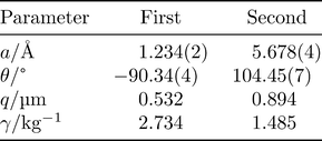
siunitx also provides an S column type that aligns numbers by their decimal point and typesets numbers in the same way as the \num command. Note that you have to be careful to wrap your headers in curly braces. Additionally, it’s a good idea to specify table-format for the S columns to ensure the headers are properly centered. (Otherwise, they’re centered about the decimal point.) For example:

\begin{tabular}
  {
    @{}
    >{$}l<{$}
    S[table-format=-2.3(1)]
    S[table-format=3.3(1)]
    @{}
  }
  \toprule
  {\text{Parameter}} & {First} & {Second} \\
  \midrule
  a / \si{\angstrom} & 1.234(2) & 5.678(4) \\
  \theta / \si{\degree} & -90.34(4) & 104.45(7) \\
  q / \si{\micro\meter} & 0.532 & 0.894 \\
  \gamma / \si{\per\kilo\gram} & 2.734 & 1.485 \\
  \bottomrule
\end{tabular}

yields

Graphics

The graphicx package works well for including most types of external images (e.g. JPG, PNG, EPS, PDF) but does not have support for SVG images.

The svg package makes it easy to include SVG images by converting them to PDFs with Inkscape. It also makes it possible to compile the text in your SVGs with LaTeX so the formatting of the text and equations matches your document. Note that using MS Windows requires some special configuration and using the subcaption package requires a workaround. Also note that on all platforms, you need to use the -shell-escape option with pdfLaTeX for this to work. For example, if you’re using a Makefile with latexmk, then you could write your rule like this:

%.pdf: %.tex $(wildcard *.svg)
	latexmk -pdf -pdflatex="pdflatex -shell-escape %O %S" "$<"

The tikz package is great for drawing complex technical diagrams that would be difficult to draw by other means. As a nice bonus, the source of the diagram is plain text, so it works well with version control. For example, I drew this image with tikz:

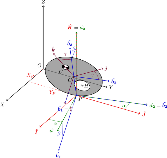
You can find many additional examples at TeXample.net.

Often, the best way to include a tikz image in your document is to create it in a separate file, and then include it with the standalone package. This way, you can render the image by itself quickly while you’re editing it, and your main document stays clean.

Captions

I prefer the captions to be smaller than the body text. You can achieve this with the caption package. It also provides the \captionof command, which is useful for cover pages. Include the package like this to get small captions:

\usepackage[font=small]{caption}

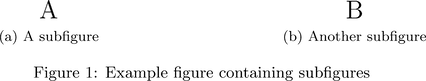
Often, it’s useful to have multiple subfigures/subtables make up an overall figure/table and be able to label/cross-reference the subfigures/subtables individually. The subcaption package works well for this, in particular the subfigure/subtable environments and the \subcaptionbox command. Include the package like this:

\usepackage{subcaption}

Here’s an example of using the subfigure environment:

Note that if you use the subcaption package with the svg package, you need to add the following to your preamble (before including svg) to avoid conflicts between the packages:

\usepackage{scrlfile}
\PreventPackageFromLoading{subfig}

Table Formatting

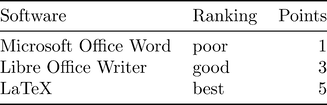
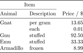
The booktabs package makes it easy to generate professional-looking tables with a minimum of effort (only three commands for most tables), such as this one:

Here’s a more complex example from the documentation:

In some cases, the tabu package is easier to use than the built-in LaTeX tabular environment, such as when creating tables inside of equations.

Code Listings

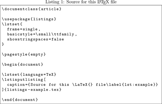
Use the listings package. It allows you to include external files as code listings, easily cross-reference the listings, and format the listings nicely. This is how I like include the package:

\usepackage{listings}
\lstset{frame=single,basicstyle=\small\ttfamily,showstringspaces=false}

and here’s an example of the output:

Hyperlinks, URLs, and PDF Metadata

Use the hyperref package to automatically create links for cross-references, to allow you create external links to URLs, and to allow you to edit the metadata of the output PDF. For example, I include the hyperref package like this (I define \thetitle and \theauthor elsewhere):

\usepackage[unicode,xetex]{hyperref}
\hypersetup{
  colorlinks,
  citecolor = black,
  filecolor = black,
  linkcolor = black,
  urlcolor = black,
  pdftitle = \thetitle,
  pdfauthor = \theauthor,
  pdfdisplaydoctitle = true
}

You can create a hyperlinked URL like this: \url{https://archive.org}, and you can create a named external link like this: \href{https://archive.org}{Internet Archive}.

Cross-Referencing

The cleveref package makes it easy to correctly format cross references. For example, you can write \cref{fig:foo,fig:bar} instead of figures~\ref{fig:foo} and~\ref{fig:bar}. I change the \creflastjunction from the default to add a serial comma:

\usepackage{cleveref}
\newcommand{\creflastconjunction}{, and~}

Note that you must include the cleveref package after you include the hyperref package.

Header and Footer

I like to have a fancy header that gives the current section, document title, and author’s name. I use the fancyhdr package:

\usepackage{fancyhdr}
\fancyhf{}
\fancyhead[L]{\leftmark}
\fancyhead[C]{\MakeUppercase{\thetitle}}
\fancyhead[R]{\MakeUppercase{\theauthor}}
\fancyfoot[C]{\thepage}
\pagestyle{fancy}